2. First Steps¶

2.1.1. Launching IPython¶

Once you have installed Python, open a shell and at the prompt type:

$ cd ~
$ mkdir testfold
$ cd testfold

which will make a new directory called testfold and change into it.

By typing short commands at the prompt, IPython can be used to perform various system tasks, such as running programs and creating and moving files around on your computer. This is a different kind of computer interface than the icon-based interface (or “graphical user interface” GUI) that you usually use to communicate with your computer. While it may seem more cumbersome for some tasks, it can be more powerful for other tasks, particularly those associated with programming.

Before getting started, we point out that like most modern computer languages, Python is case sensitive. That is, Python distinguishes between upper and lower case letters. Thus, two words spelled the same but having different letters capitalized are treated as different names in Python. Keep that in mind as we introduce different commands.

2.1.2. Testing your installation of Python¶

Running the Python program below tests your installation of Python to verify that the installation was successful. In particular, it tests that the NumPy, SciPy, and MatPlotLib libraries that are needed for this manual are properly installed. Now that you are in directory testfold, start a python session with:

$jupyter  qtconsole &

The ‘&’ at the end ‘backgrounds’ the session and gives you back the bash prompt so you can type further commands.

Launch atom from the command line with the empty file name test_python.py:

$ atom test_python.py

Copy these lines into test_python.py You should input your first and last names inside the single quotes on lines 15 and 16, respectively. Save this file in atom.

 1
 2
 3
 4
 5
 6
 7
 8
 9
10
11
12
13
14
15
16
17
18
19
20
21
22
23
24
25
26
27
28
29
30
31
32
33
34
35
36
37
38
39
40
41
42
43
44
45
46
47
48

# This code tests that your Python installation worked.
# It generates a png image file that you should e-mail
# to the address shown on the plot
import scipy
import numpy
import matplotlib
import matplotlib.pyplot as plt
import platform
import socket

# If you are a student, please fill in your first and last
# names inside the quotes in the two lines below.  Do not
# modify anything else in this file

your_first_name = 'First'
your_last_name = 'Last'

# If you are an instructor, modify the next 3 lines.
# You do not need to modify anything else in this file.

classname = 'ATSC 301'
term = 'Fall_2016'      # must contain no spaces
email = 'paustin@eos.ubc.ca'

plt.plot([0,1], 'r', [1,0], 'b')
plt.text( 0.5, 0.8, '{0:s} {1:s}'
        .format(your_first_name, your_last_name),
        horizontalalignment='center',
        size = 'x-large',
        bbox=dict(facecolor='purple', alpha=0.4))
plt.text( 0.5, 0.1,
    '{1:s}\nscipy {2:s}\nnumpy {3:s}\nmatplotlib {4:s}\non {5:s}\n{6:s}'
        .format(
        classname,
        term,
        scipy.__version__,
        numpy.__version__,
        matplotlib.__version__,
        platform.platform(),
        socket.gethostname()
        ) ,
    horizontalalignment='center'
    )
filename = your_last_name + '_' + your_first_name + '_' + term + '.png'
plt.title('*** E-mail the saved version of this plot, ***\n' +
    '"{0:s}" to {1:s}'.format(filename, email), fontsize=12)
plt.savefig(filename)
plt.show()

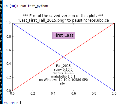
To run your saved file go to the IPython window and at the prompt type:

run test_python

which should produce a plot that looks something like this:

To save this as a png file, type:

%matplotlib qt4

which switches from inline graphics to graphics that appear in a separate window. Type:

run test_python

again to get a windowed plot

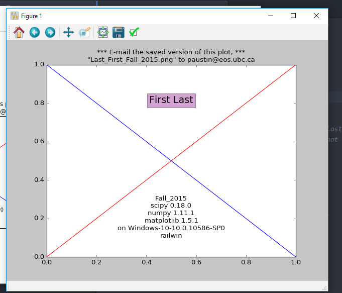
Clicking on the floppy disk icon should prompt you for a file name to save the figure into.

2.2.1. Magic Functions¶

IPython features a number of commands called “magic” commands that let you perform various useful tasks. There are two types of magic commands, line magic commands that begin with %—these are executed on a single line—and cell magic commands that begin with %%—these are executed on several lines. Here we will concern ourselves only with line magic commands.

The first thing to know about magic commands is that you can toggle (turn on and off) the need to use the % prefix for line magic commands by typing %automagic. By default, the Automagic switch is set to ON so you don’t need the % prefix. To set Automagic to OFF, simply type %automagic at the IPython prompt. Cell magic commands always need the %% prefix.

In what follows below, we assume that the Automagic switch is set to ON so we omit the % sign.

2.2.2. Navigation Commands¶

IPython recognizes several common navigation commands that are used under the Unix/Linux operating systems. In the IPython shell, these few commands work on Macs, PCs, and Linux machines.

At the IPython prompt, type cd ~ (i.e. “cd” – “space” – “tilde” , where tilde is found near the upper left part of most keyboards). This will set your computer to its home (default) directory. Next type pwd (print working directory) and press RETURN. The console should return the name of the current directory of your computer. It might look like this on a Mac:

In [2]: pwd
Out[2]: u'/Users/phil'

or this on a PC:

In [3]: pwd
Out[3]: C:\\Users\\phil

The responses Out[2]: u'/Users/phil' for the Mac and Out[3]: C:\\Users\\phil for the PC mean the the current directory is phil, which is a subdirectory of Users. Taken together /Users/phil on a Mac or C:\\Users\\phil on a PC is known as the path of the current directory. The path is just the name of a directory and the sequence of subdirectories in which it resides up to the root directory.

Typing cd .. (“cd” – “space” – two periods) moves the IPython shell up one directory in the directory tree, as illustrated by the set of commands below.

In [4]: cd ..
/Users

In [5]: pwd
Out[5]: u'/Users'

The directory moved up one from /Users/phil to /Users. Now type ls (list) and press RETURN. The console should list the names of the files and subdirectories in the current directory.

In [6]: ls
Shared/    phil/

In this case, there are only two directories (indicated by the slash) and not files. Type cd ~ again to return to your home directory and then type pwd to verify where you are in your directory tree. [Technically, ls isn’t a magic command, but typing it without the % sign lists the contents of the current directory, irrespective of whether Automagic is ON or OFF.]

Let’s create a directory within your documents directory that you can use to store your Python programs. We will call it PyProgs. First, return to your home directory by typing cd ~. To create directory PyProgs, type mkdir PyProgs (make directory). Type ls to confirm that you have created PyProgs and then type cd PyProgs to switch to that directory.

Now let’s say you want to return to the previous subdirectory, Documents or My Documents, which should be one up in the directory tree if you have followed along. Type cd .. and then type pwd. You should find that you are back in the previous directory, Documents or My Documents. If you type ls, you should see the new directory PyProgs that you just created.

2.2.3. More Magic Commands¶

The most important magic command is %run filename where filename is the name of a Python program you have created. We haven’t done this yet but include it here just for reference. We will come back to this later.

Some other useful magic commands include %hist, which lists the recent commands issued to the IPython terminal, and %edit, which opens a new empty file in the code editor window. Typing %edit filename, will open the file filename if it exists in the current directory, or it will create a new file by that name if it does not, and will open it as a blank file in the code editor window.

There are a number of other magic commands. You can get a list of them by typing lsmagic.

In [7]: lsmagic
Available line magics:
%alias  %alias_magic  %autocall  %automagic  %bookmark  %cd
%clear  %colors  %config  %connect_info  %debug  %dhist  %dirs
%doctest_mode  %ed  %edit  %env  %gui  %guiref  %hist  %history
%install_default_config  %install_ext  %install_profiles
%killbgscripts  %less  %load  %load_ext  %loadpy  %logoff  %logon
%logstart %logstate  %logstop  %lsmagic  %macro  %magic  %man
%more  %notebook  %page  %pastebin  %pdb  %pdef  %pdoc  %pfile
%pinfo  %pinfo2  %popd  %pprint  %precision  %profile  %prun
%psearch  %psource  %pushd  %pwd  %pycat  %pylab  %qtconsole
%quickref  %recall  %rehashx  %reload_ext  %rep  %rerun  %reset
%reset_selective  %run  %save  %sc  %store  %sx  %system  %tb
%time  %timeit  %unalias  %unload_ext  %who  %who_ls  %whos
%xdel  %xmode

Available cell magics:
%%!  %%bash  %%capture  %%file  %%javascript  %%latex  %%perl
%%prun  %%pypy %%python  %%python3  %%ruby  %%script  %%sh  %%svg
%%sx  %%system  %%timeit

Automagic is ON, % prefix IS NOT needed for line magics.

There are a lot of magic commands, most of which we don’t need right now. We will introduce them in the text as needed.

2.2.4. System shell commands¶

You can also run system shell commands from the IPython shell by typing ! followed by a system shell command. For Macs running OSX and for Linux machines, this means that Unix (or equivalently Linux) commands can be issued from the IPython prompt. For PCs, this means that Windows (DOS) commands can be issued from the IPython prompt. For example, typing !ls (list) and pressing RETURN lists all the files in the current directory on a Mac. Typing !dir on a PC does essentially the same thing (note that system shell commands in Windows are not case sensitive).

2.2.5. Tab completion¶

IPython also incorporates a number of shortcuts that make using the shell more efficient. One of the most useful is tab completion. Let’s assume you have been following along and that your are in the directory Documents or My Documents. To switch to the directory PyProgs, you could type cd PyProgs. Instead of doing that, type cd PyP and then press the TAB key. This will complete the command, provided there is no ambiguity in how to finish the command. In the present case, that would mean that there was no other subdirectory beginning with PyP. Tab completion works with any command you type into the IPython terminal. Try it out! It will make your life more wonderful.

A related shortcut involves the \(\uparrow\) key. If you type a command, say cd and then to press the \(\uparrow\) key, IPython will complete the cd command with the last instance of that command. Thus, when you launch IPython, you can use this shortcut to take you to the directory you used when you last ran IPython.

You can also simply press the \(\uparrow\) key, which will simply recall the most recent command. Repeated application of the \(\uparrow\) key scrolls though the most recent commands in reverse order. The \(\downarrow\) key can be used to scroll in the other direction.

2.2.6. Recap of commands¶

Let’s recap the (magic) commands introduced above:

pwd:

(print working directory) Prints the path of the current directory.

ls:

(list) Lists the names of the files and directories located in the current directory.

mkdir filename:

(make directory) Makes a new directory filename.

cd directoryname:

(change directory) Changes the current directory to directoryname. Note: for this to work, directoryname must be a subdirectory in the current directory. Typing cd ~ changes to the home directory of your computer. Typing cd .. moves the console one directory up in the directory tree.

clear:

Clears the IPython screen of previous commands.

run filename:

Runs (executes) a Python script. Described later in the section Scripting Example 1

Tab completion:

Provides convenient shortcuts, with or without the arrow keys, for executing commands in the IPython shell.

2.3.1. Binary arithmetic operations in Python¶

The table below lists the binary arithmatic operations in Python. It has all the standard binary operators for arithmetic, plus a few you may not have seen before.

Operation	Symbol	Example	Output
addition	+	12+7	19
subtraction	-	12-7	5
multiplication	*	12*7	84
division	/	12/7	1.714285
floor division	//	12//7	1
remainder	%	12%7	5
exponentiation	**	12**7	35831808

Floor division, designated by the symbols //, means divide and keep only the integer part without rounding. Remainder, designated by the symbols %, gives the remainder of after a floor division.

One peculiarity of all versions of Python prior to version 3 is that dividing two integers by each other yields the “floor division” result—another integer. Therefore 12/7 yields 1 whereas 12./7 or 12/7. or 12./7. all yield 1.714285. Starting with version 3 of Python, all of the above expressions, including 3/2 yield 1.714285. Unfortunately, we are using version 2.7 of Python so 12/7 yields 1. You can force versions of Python prior to version 3 to divide integers like version 3 does by typing

from __future__ import division

at the beginning of an IPython session. You only need to type it once and it works for the entire session.

2.3.2. Types of numbers¶

There are four different types of numbers in Python: plain integers, long integers, floating point numbers, and complex numbers.

Plain integers, or simply integers, are 32 bits (binary digits) long, which means they extend from \(-2^{31}=-2147483648\) to \(2^{31}-1=2147483647\). One bit is used to store the sign of the integer so there are only 31 bits left—hence, the power of 31. In Python, a number is automatically treated as an integer if is written without a decimal point and it is within the bounds given above. This means that 23, written without a decimal point, is an integer and 23., written with a decimal point, is a floating point number. If an integer extends beyond the bounds of a simple integer, the it becomes a long integer, and is designated as such by an L following the last digit. Here are some examples of integer arithmetic:

In [4]: 12*3
Out[4]: 36

In [5]: 4+5*6-(21*8)
Out[5]: -134

In [6]: 11/5
Out[6]: 2.2

In [7]: 11//5
Out[7]: 2

In [8]: 9734828*79372    # product of these two large integers
Out[8]: 772672768016L    # is a long integer

For the binary operators +, -, *, and //, the output is an integer if the inputs are integers. The only exception is if the result of the calculation is out of the bounds of Python integers, in which case Python automatically converts the result to a long integer. The output of the division operator / is a floating point as of version 3 of Python. If an integer output is desired when two integers are divided, the floor division operator // must be used.

Floating point numbers are essentially rational numbers and can have a fractional part; integers, by their very nature, have no fractional part. In most versions of Python running on PCs or Macs, floating point numbers go between approximately \(\pm 2 \times 10^{-308}\) and \(\pm 2 \times 10^{308}\). Here are some examples of floating point arithmetic:

In [9]: 12.*3.
Out[9]: 36.0

In [10]: 123.4*(-53.9)/sqrt(5.)
Out[10]: -2974.5338992050501

In [11]: 11./5.
Out[11]: 2.2

In [12]: 11.//5.
Out[12]: 2.0

In [13]: 11.%5.
Out[13]: 1.0

In [14]: 6.022e23*300.
Out[14]: 1.8066e+26

Note that the result of any operation involving only floating point numbers as inputs is a real number, even in the cases where the floor division // or remainder % operators are used. The last output also illustrates an alternative way of writing floating point numbers as a mantissa followed by and e or E followed by a power of 10: so 1.23e-12 is equivalent to \(1.23 \times 10^{-12}\).

We also sneaked into our calculations sqrt, the square root function. We will have more to say about functions in a few pages.

Complex numbers are written in Python as a sum of a real and imaginary part. For example, the complex number \(3-2i\) is represented as 3-2j in Python where j represents \(\sqrt{-1}\). Here are some examples of complex arithmetic:

In [15]: (2+3j)*(-4+9j)
Out[15]: (-35+6j)

In [16]: (2+3j)/(-4+9j)
Out[16]: (0.1958762886597938-0.3092783505154639j)

In [17]: sqrt(-3)
Out[17]: nan

In [18]: sqrt(-3+0j)
Out[18]: 1.7320508075688772j

Notice that to obtain the expected result or \(\sqrt{-3}\), you must write the argument of the square root function as a complex number. Otherwise, Python returns nan (not a number).

If you multiply an integer by a floating point number, the result is a floating point number. Similarly, if you multiply a floating point number by a complex number, the result is a complex number. Python always promotes the result to the most complex of the inputs.

2.5.1. Some NumPy functions¶

NumPy includes an extensive library of mathematical functions. In the table below, we list some of the most useful ones. A much more complete list is available at http://docs.scipy.org/doc/numpy/reference/ufuncs.html#math-operations.

Function	Description
sqrt(x)	Square root of \(x\)
exp(x)	Exponential of x, i.e. \(e^{x}\)
log(x)	Natural log of x, i.e. \(\ln x\)
log10(x)	Base 10 log of \(x\)
degrees(x)	Converts \(x\) from radians to degrees
radians(x)	Converts \(x\) from degrees to radians
sin(x)	Sine of \(x\) (\(x\) in radians)
cos(x)	Cosine \(x\) (\(x\) in radians)
tan(x)	Tangent \(x\) (\(x\) in radians)
arcsin(x)	Arc sine (in radians) of \(x\)
arccos(x)	Arc cosine (in radians) of \(x\)
arctan(x)	Arc tangent (in radians) of \(x\)
fabs(x)	Absolute value of \(x\)
round(x)	Rounds a float to nearest integer
floor(x)	Rounds a float down to nearest integer
ceil(x)	Rounds a float up to nearest integer
sign(x)	-1 if \(x<0\), +1 if \(x>0\), 0 if \(x=0\)

The functions discussed here all have one input and one output. Python functions can, in general, have multiple inputs and multiple outputs. We will discuss these and other features of functions later when we take up functions in the context of user-defined functions.

2.5.2. Keyword arguments¶

In addition to regular arguments, Python functions can have keyword arguments (kwargs). Keyword arguments are optional arguments that need not be specified when a function is called. See Basic plotting for examples of the use of keyword arguments. For the moment, we don’t need them so we defer a full discussion of keyword arguments until we introduce them in the section on User-defined functions.

2.6.1. Names and the assignment operator¶

A variable is a name that is used to store data. It can be used to store different kinds of data, but here we consider the simplest case where the data is a single numerical value. Here are a few examples:

In [1]: a = 23

In [2]: p, q = 83.4, sqrt(2)

The equal sign “=” is the assignment operator. In the first statement, it assigns the value of 23 to the variable a. In the second statement it assigns a value of 83.4 to p and a value of 1.4142135623730951 to q. To be more precise, the name of a variable, such as a, is associated with a memory location in your computer; the assignment variable tells the computer to put a particular piece of data, in this case a numerical value, in that memory location. Note that Python stores the numerical value, not the expression used to generate it. Thus, q is assigned the 17-digit number 1.4142135623730951 generated by evaluating the expression sqrt(2), not with \(\sqrt{2}\). (Actually the value of q is stored as a binary, base 2, number using scientific notation with a mantissa and an exponent.)

Suppose we write

In [3]: b = a

In this case Python associates a new memory location with the name b, distinct from the one associated with a, and sets the value stored at that memory location to 23, the value of a. The following sequence of statements demonstrate that fact. Can you see how? Notice that simply typing a variable name and pressing Return prints out the value of the variable.

In [4]: a=23

In [5]: b=a

In [6]: a
Out[6]: 23

In [7]: b
Out[7]: 23

In [8]: a=12

In [9]: a
Out[9]: 12

In [10]: b
Out[10]: 23

The assignment variable works from right to left; that is, it assigns the value of the number on the right to the variable name on the left. Therefore, the statement “5=a” makes no sense in Python. The assignment operator “=” in Python is not equivalent to the equals sign “\(=\)” we are accustomed to in algebra.

The assignment operator can be used to increment or change the value of a variable

In [11]: b = b+1

In [12]: b
Out[12]: 24

The statement, b = b+1 makes no sense in algebra, but in Python (and most computer languages), it makes perfect sense: it means “add 1 to the current value of b and assign the result to b.” This construction appears so often in computer programming that there is a special set of operators to perform such changes to a variable: +=, -=, *=, and /=. Here are some examples of how they work:

In [13]: c , d = 4, 7.92

In [14]: c += 2

In [15]: c
Out[15]: 6

In [16]: c *= 3

In [16]: c
Out[16]: 18

In [17]: d /= -2

In [17]: d
Out[17]: -3.96

In [18]: d -= 4

In [19]: d
Out[19]: -7.96

Verify that you understand how the above operations work.

2.6.2. Legal and recommended variable names¶

Variable names in Python must start with a letter, and can be followed by as many alphanumeric characters as you like. Spaces are not allowed in variable names. However, the underscore character “_” is allowed, but no other character that is not a letter or a number is permitted.

Recall that Python is case sensitive, so the variable a is distinct from the variable A.

We recommend giving your variables descriptive names as in the following calculation:

In [20]: distance = 34.

In [21]: time_traveled = 0.59

In [22]: velocity = distance/time_traveled

In [23]: velocity
Out[23]: 57.6271186440678

The variable names distance, time_traveled, and velocity immediately remind you of what is being calculated here. This is good practice. But so is keeping variable names reasonably short, so don’t go nuts!

2.6.3. Reserved words in Python¶

There are also some names or words that are reserved by Python for special purposes or functions. You must avoid using these names, which are provided here for your reference:

and	del	from	not	while
as	elif	global	or	with
assert	else	if	pass	yield
break	except	import	print
class	exec	in	raise
continue	finally	is	return
def	for	lambda	try

In addition, you should not use function names, like sin, cos, and sqrt, defined in the SciPy, NumPy, or any other library that you are using.

2.7.1. Scripting Example 1¶

Let’s work through an example to see how scripting works. Suppose you are going on a road trip and you would like to estimate how long the drive will take, how much gas you will need, and the cost of the gas. It’s a simple calculation. As inputs, you will need the distance of the trip, your average speed, the cost of gasoline, and the mileage of your car.

Writing a script to do these calculations is straightforward. First, launch Spyder and open the code editor. Enter the following in the editor pane:

# Calculates time, gallons of gas used, and cost of gasoline for
# a trip
distance = 400.         # miles
mpg = 30.               # car mileage
speed = 60.             # average speed
costPerGallon = 4.10    # price of gas

time = distance/speed
gallons = distance/mpg
cost = gallons*costPerGallon

The number (or hash) symbol # is the “comment” character in Python; anything on a line following # is ignored when the code is executed. Judicious use of comments in your code will make your code much easier to understand days, weeks, or months after the time you wrote it. Use comments generously.

Python ignores blank spaces or “white space” as it is sometimes called. The statement costPerGallon = 4.10 in the above program could equally well be written as costPerGallon=4.10 without the spaces before and after the = assignment operator; either way the statement means the same thing. Similarly, the white space after costPerGallon = 4.10 but before the comment (hash) symbol is also ignored by Python. The idea is that you should use white space to make your program more readable.

Now you are ready to run the code.

In [1]: cd ~/Documents/PyProgs/

To run or execute a script, simply type run filename, which in this case means type run myTrip.py. When you run a script, Python simply executes the sequence of commands in the order they appear.

In [2]: run myTrip.py

Once you have run the script, you can see the values of the variables calculated in the script simply by typing the name of the variable. IPython responds with the value of that variable.

In [3]: time
Out[3]: 6.666666666666667

In [4]: gallons
Out[4]: 13.333333333333334

In [5]: cost
Out[5]: 54.666666666666664

You can change the number of digits IPython displays using the command %precision:

In [6]: %precision 2
Out[6]: u'%.2f'

In [7]: time
Out[7]: 6.67

In [8]: gallons
Out[8]: 13.33

In [9]: cost
Out[9]: 54.67

Typing %precision returns IPython to its default state; %precision %e causes IPython to display numbers in exponential format (scientific notation).

print(time)
print(gallons)
print(cost)

2.7.2. Scripting Example 2¶

Let’s try another problem. Suppose you want to find the distance between two Cartesian coordinates \((x_1, y_1, z_1)\) and \((x_2, y_2, z_2)\). The distance is given by the formula

Now let’s write a script to do this calculation and save it in a file called twoPointDistance.py.

1
2
3
4
5
6
7

# Calculates the distance between two 3d Cartesian coordinates
import numpy as np

x1, y1, z1 = 23.7, -9.2, -7.8
x2, y2, z2 = -3.5, 4.8, 8.1

dr = np.sqrt( (x2-x1)**2 + (y2-y1)**2 + (z2-z1)**2 )

We have introduced extra spaces into some of the expressions to improve readability. They are not necessary; where and whether you include them is largely a matter of taste.

There are two important differences between the code above and the commands we would have written into the IPython console to execute the same set of commands. The first is the statement on the second line

...
import numpy as np
...

and the second is the “np.” in front of the sqrt function on the last line. If you leave out the import numpy as np line and remove the np. in front of the sqrt function, you will get the following error message

----> 7 dr = sqrt( (x2-x1)**2 + (y2-y1)**2 + (z2-z1)**2 )

NameError: name 'sqrt' is not defined

The reason for the error is that the sqrt function is not a part of core Python. But it is a part of the NumPy module discussed earlier. To make the NumPy library available to the script, you need to add the statement import numpy as np. Then, when you call a NumPy function, you need to write the function with the np. prefix. Failure to do either will result in a error message. Now we can run the script.

In [10]: run twoPointDistance.py

In [11]: dr
Out[11]: 34.48

The script works as expected.

The reason we do not have to import NumPy when working in the IPython shell is that it is done automatically when the IPython shell is launched. Similarly, the package MatPlotLib is also automatically loaded (imported) when IPython is launched. However, when a script or program is executed, it is run on its own outside the IPython shell, even if the command to run the script is executed from the IPython shell.

dr = np.sqrt( (x2-x1)**2
            + (y2-y1)**2
            + (z2-z1)**2 )

a = 1 + 2 \
  + 3 + 4

a = 1 + 2 + 3 + 4